Solving a 2D Poisson equation with Neumann boundary
conditions through discrete Fourier cosine transform
by JARNO ELONEN (elonen@iki.fi),
21.12.2004
The book NUMERICAL RECIPIES IN
C, 2ND EDITION (by PRESS,
TEUKOLSKY, VETTERLING &
FLANNERY) presents a recipe for solving a
discretization of 2D Poisson equation
 numerically by Fourier transform ("rapid solver"). While
it shows the explicit solution for the problem with several other
boundary conditions, Neumann condition
numerically by Fourier transform ("rapid solver"). While
it shows the explicit solution for the problem with several other
boundary conditions, Neumann condition
 is
handled quite briefly. The following demonstrates in detail how
to derive an equation for
is
handled quite briefly. The following demonstrates in detail how
to derive an equation for
 using
the definition of the inverse Fourier cosine transform. The
solution turns out, perhaps not very surprisingly, to be exacly
the same as for the sine transform.
using
the definition of the inverse Fourier cosine transform. The
solution turns out, perhaps not very surprisingly, to be exacly
the same as for the sine transform.
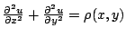
The finite difference equation is:
...from which we need to solve  . First, some abbreviations:
Now, the inverse 2D discrete cosine transform is:
Substitute this to both sides of the above finite difference
equation and remove the summation to obtain:
Using the following lemmas...
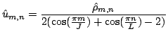
...we simplify and solve for
 :
:
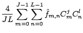
Hence, to solve the Poisson equation, first compute the 2D cosine
transform
 ,
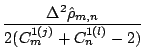
then calculate...
...and finally do an inverse cosine transform to obtain
. In
practice, when the denominator becomes 0, substitute it with some
small
,
then calculate...
...and finally do an inverse cosine transform to obtain
. In
practice, when the denominator becomes 0, substitute it with some
small  to avoid division by zero.